Playing Atari Through Deep Reinforcement Learning.

March 3, 2020 9 minute read

AbstractPermalink

In this project, I experiment with the Deep Q Networks on Atari Environment. These networks are able to learn policies from the input using reinforcement Learning. The network is trained with a variant of Q-learning, with input as raw pixels from the screen and the output is action value function which estimates future rewards for each action.

2) IntroductionPermalink

Learning control policies directly from images or some other high dimensional sensory input was not possible before the advent of deep learning. However, even with deep learning at our disposal, there are several challenges in applying to solve reinforcement learning problems. Deep Learning methods require large amounts of training data and how that can be mapped to a reinforcement learning problem is not immediately clear. One might argue to learn a model of the environment by estimating transition probabilities and reward functions but that is almost impossible for most environments due to very large state space and stochasticity in the system. Another issue with deep learning-based methods is that we need our training samples to be independent whereas in reinforcement learning, we get a sequence of states which have high correlation between them. Deep Q Networks [1], along with a variant of Q-learning [2] helps us to tackle these challenges.

2) BackgroundPermalink

In this project, I will be experimenting with Atari environment [3], specifically the Space Invaders environment. (However, the implementation is well organized to be able to tackle other environments as well with minor modifications that will be needed as per the dynamics of different environments). In general, any reinforcement learning problem with single agent consists of an environment, and at each time step, the agent selects an action at from the agent’s action space. (There are 6 actions in Space Invaders environment. ${0: no \; action}$

${1: fire}$

${2: move\;right}$

${3: move\;left}$

${4: move\;right\;fire}$

${5: move \;left \; fire})$

The agent gets to only observe the images of the current screen frame ${x_t}$ . The The goal of the agent is to interact with the environment by selecting actions in a way that maximizes future rewards. I have considered discounted rewards such that the discounted return at time $t$ can be written as ${R_t = \sum_{t'=1}^{T}{\gamma^{t'-t} r_t} }$ where T is the time-step at which the game ends.

We can also define the optimal action value function, which can be defined as the maximum expected reward achievable by following an optimal policy, using Bellman equation as follows.

$\DeclareMathOperator{\E}{\mathbb{E}} \begin{equation} Q^*(s,a) = \E_{s'\sim \mathcal{E}}\;\left[r+ \gamma\underset{a'}{max}Q^*(s',a')|s,a \right] \end{equation}$

In this project, this action value function is estimated using a neural network as a function approximator. We can use one neural network for each action or alternatively use one single neural network that will approximate the action value function for each action.

$\DeclareMathOperator{\E}{\mathbb{E}} \begin{equation} Q(s,a;\theta) \approx Q^*(s,a) \end{equation}$

This network can be trained by minimizing a sequence of loss functions $L_i(\theta_i)$ that changes at each iteration $i$ .

$\DeclareMathOperator{\E}{\mathbb{E}} \begin{equation} L_i(\theta_i) =\E_{s,a\sim p(.)}\;\left[(y_i - Q(s,a;\theta))^2 \right] \end{equation}$

where

$\begin{equation} y_i=Q^*(s,a) =\E_{s'\sim \mathcal{E}}\;\left[r+ \gamma\underset{a'}{max}Q^*(s',a')|s,a \right] \end{equation}$

is the target for iteration $i$ and ${\rho(s,a)}$ is a probability distribution over sequences ${s}$ and actions ${a}$ that the authors of the original paper referred to as behavior distribution. One important thing to note is that target depends on the network weights which is in contrast with what the target is in supervised learning, which are fixed for all iterations during training. Now, if we differentiate the loss function with respect to the weights, then the gradient can be written as follows.

$\DeclareMathOperator{\E}{\mathbb{E}} \begin{equation} \nabla_{\theta_i} L_i(\theta_i) =\E_{s,a\sim p(.);s'\sim\mathcal{E}}\;\left[\left(r+\gamma\underset{a'}{max}Q(s',a';\theta_{i-1})-Q(s,a;\theta_i) \right)\nabla_{\theta_i}Q(s,a;\theta_i) \right] \end{equation}$

However, how can we compute these gradients practically? It is computationally infeasible to calculate the full gradients and hence we use stochastic gradient descent to compute them This algorithm is same as the $Q{\text-}Learning$ algorithm. Some important things to note are that this algorithm as $model{\text-}free$ , which means that we don’t estimate the dynamics of the environment and instead solve directly from the samples. Another thing to note is that this algorithm is $off{\text-}policy$ , which means it learns an optimal policy by following a $behavior\;distribution$ . Now how to select a behavior distribution? In practice, behavior distribution is chosen to be an $\epsilon{\text-}greedy\;strategy$ which allows exploration by choosing the optimal action with probability $1{\text-}\epsilon$ and random action by probability $\epsilon$ .

3) Deep Reinforcement LearningPermalink

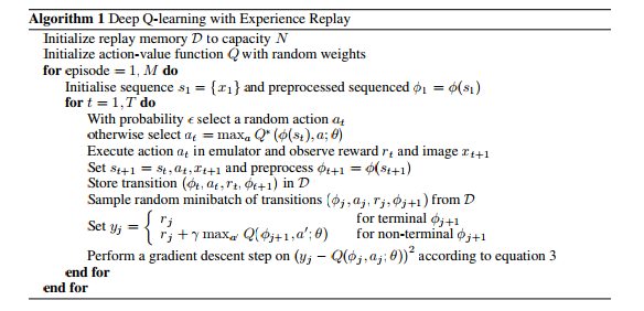
Deep Reinforcement Learning uses something called as $experience\;replay$ to store the agent’s experience at each time step as $e_t = (s_t, a_t, r_t, s_{t+1})$ in a dataset $\mathcal{D}=e_1,...,e_N$ during each episode. The weights of the network are updated using $Q{\text-}learning$ updates using samples of experience, $e\sim\mathcal{D}$ drawn at random from the experience replay dataset. After performing experience replay, the agent selects and executes action according to $\epsilon{\text-}greedy\;strategy$ . This allows for the experiences to be used in many weight updates and allows for greater data efficiency. Moreover, the samples are not correlated as the correlation is broken due to randomized sampling which acts as a training dataset for updating the network. This in turn reduces the variances of the updates. The most important thing is that, when learning $on{\text-}policy$ , the current parameters determine the next data sample that the parameters are trained on. Due to this, it is possible that the parameters might stuck in some local minima and do not converge to the desired optimal solution. Therefore, we use $off{\text-}policy\;learning$ , which in fact becomes necessary due to the use of experience replay to update the weights and not the correlated samples. The diagram below, taken from the original paper, shows the complete algorithm.

DQN Algorithm

4) Pre-Processing and Model ArchitecturePermalink

$OpenAI\;Gym$ environment for Atari games returns a RGB image as the state of the environment. However, we don’t really need colored frames to capture the information in those frames. Therefore, each frame is converted into grayscale as the first preprocessing step. Cropping of the frame, to get a $185{\text x}95$ size frame, is also done in order to capture only the relevant information. The network takes input as the processed image and outputs the action value function for each action. The network architecture consists of $1$ convolution layer and $2$ linear layers due to limited computational resources (however, one can experiment with a much more complex network in order to get much better results). The first layer is a $convolutional\;layer$ with $64$ output channels, each kernel of size $3{\text x}3$ and stride as $1$ . The second layer is a linear layer with $64$ neurons. The final layer is the output layer with number of outputs as the number of actions, the agent can perform( $6$ in the case of Space Invaders Environment).

5) ExperimentsPermalink

I have conducted experiments only on the Space Invaders environment due to limited computational resources and strict timeline. However, the network architecture is robust enough to be used for other games as well. The original paper scales all the positive rewards to be 1 and all negative rewards to be -1. However, in my implementation, I haven’t done so. I wanted to experiment with the original reward setting instead of modifying it. However, one important change that I have done, is to give a large negative reward when the episode ends. This will avoid the agent to actions which lead to end of the games or episodes. This has been done only during the learning part of the algorithm. While storing the experience into replay buffer, I have stored the original rewards without modifying them. During the training, I have used the $RMSProp\;Algorithm$ with minibatches of size $32$ . The behavior policy during training was $\epsilon{\text-} greedy$ with $\epsilon$ varied exponentially from $0.95$ to $0.05$ over a course of $500$ episodes. Since the number of episodes is very less ( restricted to this number only due to limited computational resources), the epsilon decreased only till $0.1$ . Also, the original paper decreased epsilon across each frame, whereas I have experimented by decreasing epsilon for each episode. I have also used a frame-skipping technique which is generally used for Atari games. More precisely, the agent selects actions on every $k^{th}$ frame instead of every frame, and the last action is repeated for $k$ skipped frames. I have used $k=3$ which is same as the one used by the original paper.

6) ResultsPermalink

Results

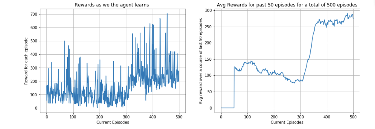
$Figure 1$ shows the results during training of the network. We can see from the plots that the agent is learning to behave in the environment in order to maximize its total expected reward.

The plot on the left in $figure 1$ shows the total reward that agent is able to get during each episode. The agent manages to achieve a maximum reward of $705$ at $456^{th}$ episode. The agent starts with taking random actions and gradually it starts choosing actions which lead to better states and hence better states. However, we can see lot of randomness in the total reward for an episode. This is due to the extreme stochastic nature of the $Space\;Invaders$ environment. In plot on the right-hand side, average rewards for past $50$ episodes has been plotted. Initially, I tried to evaluate policy after $10$ episodes. But this was computationally expensive. Therefore, I plotted the average reward for the last $50$ episodes. Important thing to note here is that the policy is changing with each episode and therefore it is not same as evaluating policy after every few episode. Nonetheless, we can see that the as the number of episodes is increasing, the average reward is also increasing which is indicating that the agent is trying to learn the optimal policy.

7) ConclusionPermalink

In this project, I explored $Deep\;Q\;Networks$ on $Atari\;Environment$ . The agent was able to learn a good enough policy and was taking actions which will lead to better rewards instead of just taking actions randomly. There were many difficulties that I had to face during this project. I read the paper on $Deep\;Q\;Networks$ to gain insights of how these networks work. In the process, I also learned about the importance of $experience\;replay$ and $off{\text-}policy\;learning$ in the case of $Deep\;Q\;Networks$ . Theoretical understanding is one thing and actually implementing is another. I faced many problems during implementation, mainly on how to divide the code into different sections to make it self-explanatory and extendable to other environments as well. If I were to start this project from scratch, I would try to extend my work to use $Deep\;Double\;Q{\text-}learning$ [3] which is an extension of $Double \;Q{\text-}Learning$ using Neural Networks. I will also try to compare the results of different algorithms across different environments. I was unable to do this in this project due to limited resources and a time constraint. But I would surely like to try out these in future.

8) ReferencesPermalink

[1] Volodymyr Mnih, Koray Kavukcuoglu, David Silver, Alex Graves, Ioannis Antonoglou, Daan Wierstra, Martin Riedmiller. Playing Atari with Deep Reinforcement Learning.

[2] Christopher JCH Watkins and Peter Dayan. Q-learning. Machine learning, 8(3-4):279–292, 1992

[3] Greg Brockman, Vicki Cheung, Ludwig Pettersson, Jonas Schneider, John Schulman, Jie Tang, Wojciech Zaremba. OpenAI Gym [4] Hado van Hasselt, Arthur Guez, David Silver. Deep Reinforcement Learning with Double Q-Learning.

Share on

Twitter Facebook LinkedIn

Sumanyu Garg