Variational Autoencoders: From A Mathematical Perspective.

1) Outline

In this post we will learn following things:

• How are Variational Autoencoders different from standard autoencoders?
• Details on the loss function of Variational Autoencoders.
• Visualizations of the latent space as we vary different parameters.

2) Recap of AutoEncoders

To fully appreciate the intriguing details of variational autoencoders, we need to begin with traditional autoencoders. Standard Autoencoders were designed for compressing the data into a smaller dimensional latent space in an unsupervised manner.

AutoEncoder Architecture

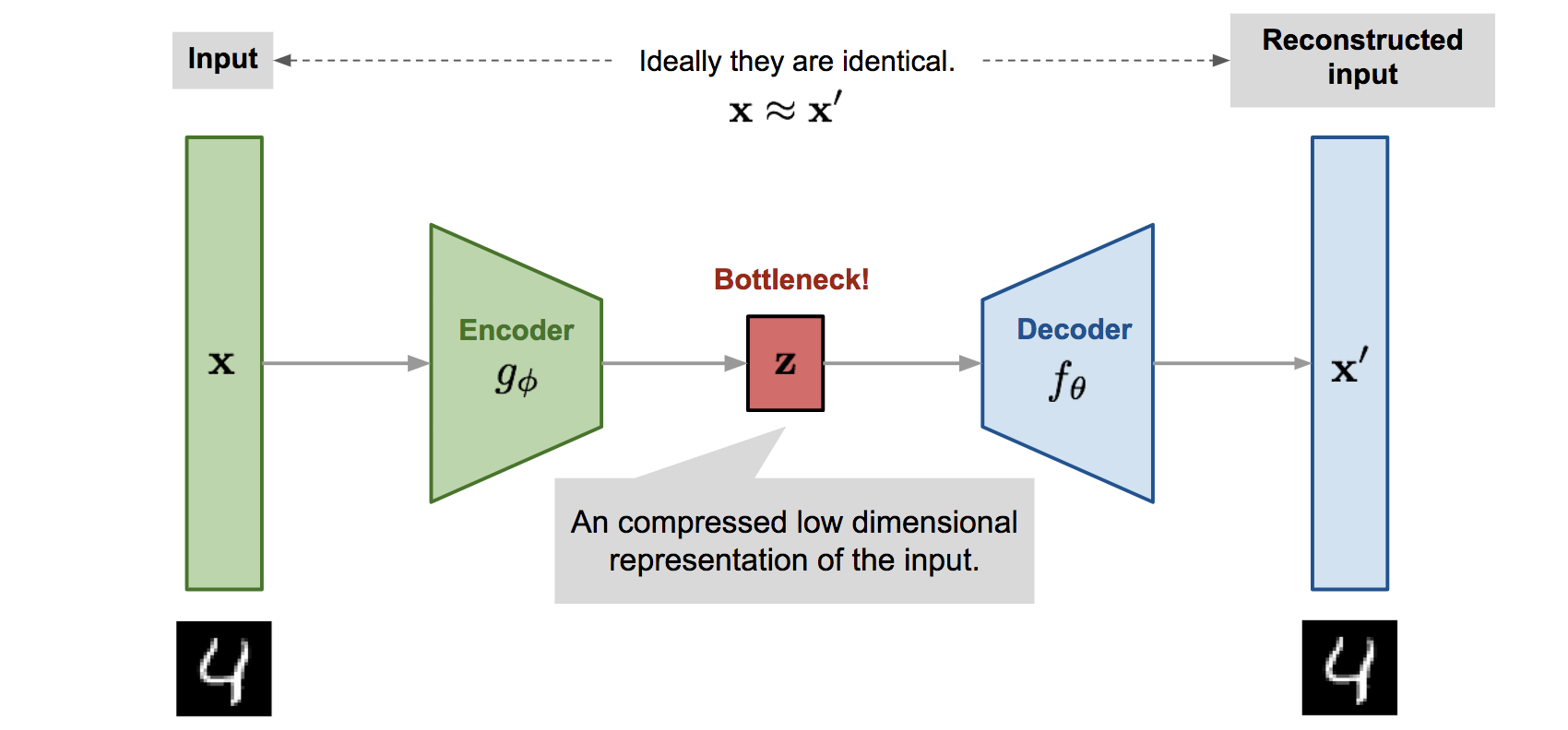
This can be achieved by having 2 functions:

1. An Encoder function \({g(x)}\), which maps the given vector \({x}\) to a hidden vector \({z}\) in a low dimensional space.
2. A Decoder function \({f(z)}\), which maps the hidden vector \({z}\) back to vector \({x}\) in original space.

One can note that in an ideal situation, \({f(z) = {g^{-1}(x)}}\)

These functions are not some arbitrary functions and will depend on the kind of data we are dealing with. Therefore, we use neural networks to approximate \(g(x)\) as \({g_\phi(x)}\) and \({f(z)}\) as \({f_\theta(z)}\) where \(\phi\) and \(\theta\) will be parameters of our encoder and decoder networks respectively. However, when we use a function approximator like neural network for approximation, \({f_\theta(z)}\) will not be exactly equal to \({g_\phi^{-1}(x)}\). Hence the output of the decoder will be an approximate vector \({x^{'}}\) in the original space which will be very similar to \({x}\).

Our objective will be to make these 2 vectors as identical to each other as possible. Therefore our optimal functions \({g_\phi(x)}\) and \({f_\theta(z)}\) will be those which minimizes the distance between these 2 vectors.

\[\begin{equation} \begin{split} \phi^{*}, \theta^{*} & = min_{\theta,\phi}\sum_{i=1}^{i=N}{\|f_\theta(g_\phi(x^{(i)}))-x^{(i)}\|^2}\\ & = min_{\theta,\phi}\sum_{i=1}^{i=N}{\|x^{'(i)}-x^{(i)}\|^2} \end{split} \end{equation}\]

Once, we have trained our autoencoder network to find optimal weights \({\phi^{*}}\) and \({\theta^*}\), we can encode a new data point in the same latent space and can also recover it back in the original space.

3) Limitations of AutoEncoders

The primary purpose of autoencoders is to compress a given vector to a lower dimensional hidden space in an unsupervised manner while preserving much of the information contained.

However, if we take any arbitrary vector from the hidden space and try to decode it using the decoder, then most likely we will simply be generating a noise. This is because the manifold mapping found out by the encoder network is not smooth (Note: Our optimization problem had no constraint to keep the hidden manifold smooth or continuous).

The encoder network just maps each vector \({x}\)​ to some location in latent space. Below figure shows the 2 dimensional latent space for MNIST Dataset. We can see that transition between different regions in the space is not continuous. Therefore, when we sample a random point from this hidden space, it will most likely correspond to a noisy point in original space.

Discontinuous Manifold in Hidden Space

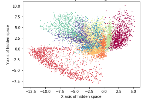
How can we obtain a meaningful representation out of an arbitrary point sampled from hidden space?

Here comes the use of Variational Encoders. In next section, we will discuss how Variational Autoencoders solve the problem of discontinuous manifold mapping to a continuous mapping so that when we sample a random point from hidden space, we generate a meaningful data point in the original space.

4) Building Blocks Towards Understanding VAE

4.1) Small background on VI and KL Divergence

In order to understand the variational autoencoders in depth, we will begin with general inference problem in Probabilistic Graphical Models(Don’t worry, everything will make sense by the end of this post in case you are wondering why we need to go to inference problem in order to understand VAE).

Consider the following setup with 2 random variables \(z(hidden)\) and \(x(observed)\) where \(z\) influences the outcome \(x\). A common problem in Bayesian Networks or probabilistic graphical models is to infer the posterior distribution of latent variable z.

Simple Probabilistic Graphical Model \[P(Z/X) = \frac{P(X/Z)}{P(X)}\]

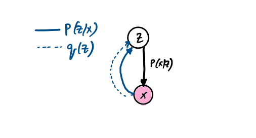
However, computing \(P(X)\) in above equation is intractable. This, means we can’t calculate posterior distribution for \(Z\). Since we cannot compute actual posterior distribution we try to approximate it. There are 2 techniques to approximate posterior.

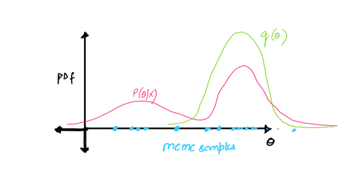
1. Markov Chain Monte Carlo (MCMC) - MCMC approach generates samples from the unnormalized \(P(Z/X)\) which in turn makes the samples unbiased. However, we need a lot of samples to approximate \(P(Z/X)\).
2. Variational Inference - Variational Inference approach approximates \(P(Z/X)\) using another distribution \(q(z)\) where \(q(z)\) belongs to some set of distributions \(Q\). This approach results in biased samples. However it is much faster and scalable to highly complex distributions \(P(Z/X)\).

Difference between MCMC and Variational Inference

(Note: I will discuss about MCMC and Variational Inference in more details in another post.)

Let’s discuss the variational inference approach in some more detail. We want to find out an approximate distribution \({q(Z)}\) which is as similar to \(P(Z/X)\). One way to measure the similarity between \(q(z)\) and \(P(Z/X)\) is to minimize the \(KL Divergence\) between these 2 distributions.

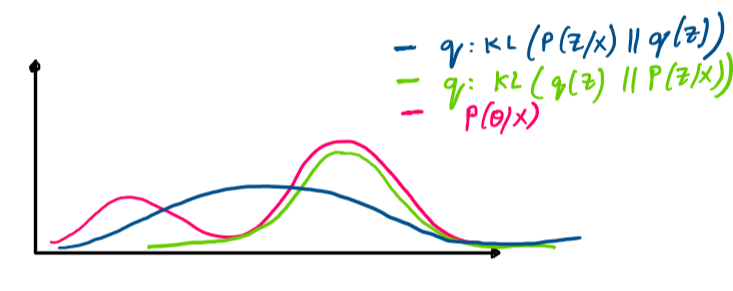
Note: We minimize \(KL(q(Z)\|P(Z/X))\) and not \(KL(P(Z/X)\|q(Z))\). Since \(KL Divergence\) is asymmetric, the 2 approaches will result in different \(q(z)\). Then why do we choose to minimize \(KL(q\|P)\) and not \(KL(P\|q)\) ?

Suppose, we restrict \(q(Z)\) to be belonging to a family of normal distributions \(Q\) , then \(q(Z)\) will be a unimodal distribution. Now, when we try to minimize \(KL(q\|P)\), then the resultant \(q(Z)\) will be a distribution which approximates one mode of \(P(Z/X)\) very well however not the others. In case, we minimize \(KL(P\|q)\), then the resultant \(q(z)\) will span across different modes of \(P(Z/X)\). When \(P(Z/X)\) is highly complex multimodal distribution, then it is better to approximate one mode in a good way rather than focusing on every mode(which essentially will result in a flat \(q(Z)\)).

Therefore, we try to minimize \(KL(q\|P)\) and not the other way around.

Different Q(Z) depending on which form of KL Divergence we minimize

4.2) Lower Bound on \(P(Z/X)\)

We want to minimize the \(KL(q(Z)\|P(Z/X))\) . Let’s try to rewrite this KL Divergence term.

\[\DeclareMathOperator{\E}{\mathbb{E}} \begin{equation} \begin{split} D_{KL}(q(Z)\|P(Z/X)) =\; & \int q(z)log(\frac{P(Z/X)}{q(Z)})\\ =\;& \int q(z)log(\frac{P(X,Z)}{P(X)q(Z)})\\ =\;& \int q(z) log(\frac{p(X,Z)}{q(Z)}) - \int q(z)log(P(X))\\ =\;&\; \int q(z) log(\frac{p(X,Z)}{q(Z)}) - log(P(X)) \end{split} \end{equation}\]

On rearranging the terms, we get the following expression,

\[\begin{equation} log(P(X)) = D_{KL}(q(Z) \| P(Z/X)) + \int q(z)log(\frac{P(X,Z)}{q(Z)}) \end{equation}\]

Now, \(log(P(X))\) is constant(as it is given to us, though we don’t know it). The first term in above equation is the quantity that we wanted to minimize. In order to minimize \(KL(q(Z)\|P(Z/X))\) , we can instead maximize the second term in the above expression i.e. \(\int q(z)log(\frac{P(X,Z)}{q(Z)})\) . Since \(KL\) is always positive, therefore,

\[\begin{equation} \int q(z)log(\frac{P(X,Z)}{q(Z)})\leq log(P(X)) \end{equation}\]

Now this term is called the Variational Lower Bound/Evidence Lower Bound on $P(X)$. We can rewrite the variational lower bound as follows:

\[\DeclareMathOperator{\E}{\mathbb{E}} \begin{equation} \begin{split} L(q) =\; & \int q(z)log(\frac{P(X,Z)}{q(Z)})\\ =\;& \int q(z)log(\frac{P(X/Z)P(Z)}{q(Z)})\\ =\;& \int q(z) log(p(X/Z)) + \int q(z)log(\frac{P(Z)}{q(Z)})\\ =\;&\; \E_{z\sim P(Z)}log(P(X/Z)) - KL(q(Z)\|P(Z)) \end{split} \end{equation}\]

Our objective has now changed to maximizing the variational lower bound \(\int q(z)log(\frac{P(X,Z)}{q(Z)})\) with respect to \(q(z)\).

\[\begin{equation} \begin{split} Objective & = \underset{q}{max}\; \int q(z)log(\frac{P(X,Z)}{q(Z)})\\ & = \underset{q}{max}\; \E_{z\sim P(Z)}log(P(X/Z)) - KL(q(Z)\|P(Z)) \end{split} \end{equation}\]

We have now finally derived the equation which we need to maximize in order to get the best lower bound on \(P(Z/X)\). Maximizing this lower bound will make \(q(Z)\) as similar to posterior \(P(Z/X)\).

5) Variational AutoEncoder:- Solving the variational lower bound equation using Neural Networks

Till now, we had been building blocks which will help us understand VAE. The basic idea behind VAE is that, we want to map the given data to a hidden space such that the manifold is continuous so that when we sample an arbitrary point from that hidden space, we are able to map it back to a meaningful data point in the actual space.

Since we want a continuous manifold, let’s assume that the mapped data points in hidden space are distributed according to distribution \(P(Z)\). And given a hidden vector \(Z=z\), the data point in original space is distributed as \(P(X/Z=z)\). Now we need to infer the posterior distribution \(P(Z/X)\).

We have discussed above that inferring true posterior is intractable, therefore we approximate true posterior using a distribution \(q(Z/X)\).

Now where does the neural network part comes in?
Neural Network at its core is function approximators and probability distributions are basically functions of random variables(with some constraints), therefore we can use Neural Networks to approximate these probability distributions by approximating the parameters of the distributions.

1. In general, we know what \(P(Z)\;\text{and}\; P(X/Z)\) are. Let \(P(Z)\) be a \(\text {normal distribution}\) with \(mean=0\;and\; variance=1\). (Choosing \(P(Z)\) and \(Q(Z/X)\) to be a \(\text {normal distributions}\), allows us to solve \(KLDivergence\) term i.e. (\(KL(q(Z)\|P(Z)\)) in closed form, though we could have chosen some other distribution as well.)

2. Similarly, we can choose \(P(X/Z)\) to be anything. However, people generally use \(P(X/Z)\) to be a \(normal\) or \(multinoulli\) distribution.

We will now write the closed form expressions for our objective functions. But before moving towards that, let’s make sure we understand the neural network architecture completely.

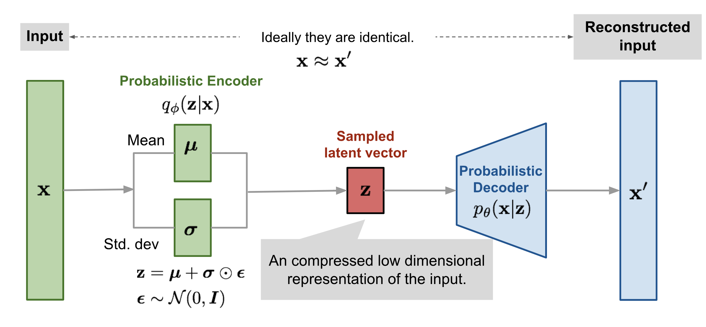
We will approximate \(P(Z/X)\) using \(q_\phi(Z/X)\) which will be a Neural Network with weights \(\phi\) . We call this the encoder part which will give us the mean and variance of \(q(Z/X)\) that maximizes our objective function.

\(P(X/Z=z)\) will be approximated by another network \(P_\theta(X/Z=z)\) where \(\theta\) represents the weights of this network and \(z\sim q_\phi(Z/X)\). This part is called the decoder network. Note, we can also make this network output mean and variance of the normal distribution representing \(P(X/Z=z)\). However, for simplicity we are just approximating the mean vector and assuming variance to be equal to 1.

6) Reparameterization Trick

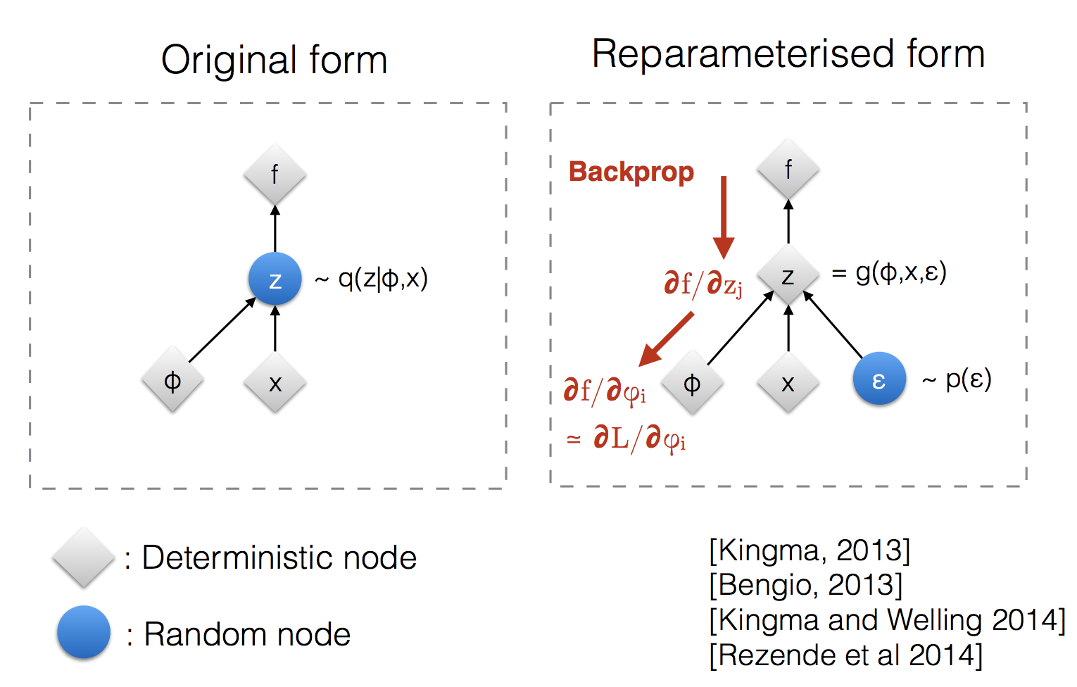
The setting which I have explained above approximates mean \(\mu\) and standard deviation \(\sigma\). Once we have \(\mu\) and \(\sigma\), we sample a \(z\) and pass it through the decoder network. However, what to do during the backpropagation stage? Sampling is a stochastic process and we cannot backpropagate gradients through a stochastic process. In order to overcome this problem, reparameterization trick is introduced. The idea is what if we shift stochastic nature to some other part of the network through which we wouldn’t need to backpropagate.

Instead of sampling \(z\) directly from \(\text{normal distribution}\) \(z^{i}\sim\;N(Z/\mu, \sigma)\), we instead sample noise from \(\epsilon^{i}\sim N(0,I)\) and transform the noise \(\epsilon^{i}\) to hidden vector \(z^{i}\). This shifts the stochastic nature of sampling to sampling from a fixed distribution through which we wouldn’t have to backpropagate.

7) Writing the loss function in closed form

Now, we have understood how variational autoencoders work. However, the objective function still looks in cryptic form. We will now simplify our objective function.

The VAE objective function can be written as follows:

\[\DeclareMathOperator{\E}{\mathbb{E}} \begin{equation} \begin{split} L(\phi, \theta) & = \underset{\theta, \phi}{max}\; \E_{z\sim q_\phi(Z/x)}log(P_\theta(X/Z)) - D_{KL}(q_\phi(Z/x) \| P(Z))\\ & = \underset{\theta, \phi}{min}\; -\E_{z\sim q_\phi(Z/x)}log(P_\theta(X/Z)) + D_{KL}(q_\phi(Z/x) \| P(Z)) \end{split} \end{equation}\]

Here, the first term is called the reconstruction loss and the second term acts as a regularizer.

• Let’s first look at the \(Kl Divergence\) term.

  ​

\[\DeclareMathOperator{\E}{\mathbb{E}} \begin{equation} \begin{split} &\; D_{KL}(q_\phi(Z/x) \| P(Z))\\ =&\;D_{KL}(N(\mu(x),\Sigma(x)) \;\;\|\;\;N(0,I))\\ =&\;\frac{1}{2}[tr(\Sigma_\phi(x))+ \mu_\phi(x)^T\mu_\phi(x)-d-log|\Sigma_\phi(x)]\\ =&\;\frac{1}{2}[\sum_{d}\Sigma_\phi(x) + \sum_{d}\mu_\phi^{2}(x)-\sum_{d}1-\sum_{d}log(\Sigma_\phi(x)]\\ =&\;\frac{1}{2}[\sum_{d}\Sigma_\phi(x) +\mu_\phi^2(x)-1-log(\Sigma_\phi(x))] \end{split} \end{equation}\]

We have now simplified the \(KlDivergence\) term in our objective function. We can now easily take derivatives with respect to \(\phi\) ,the weights of the encoder neural network. It is important to note here that the \(KL Divergence\) term is only dependent on the weights of    the encoder network and not the decoder network.

• Let’s now simplify the reconstruction loss term. Here, I have assumed that \(P_\theta(X/Z)\) follows a \(\text{normal distribution}\) with \(mean\) \(f_\theta(z)\) determined by the decoder network and \(variance\) equal to 1.

\[\DeclareMathOperator{\E}{\mathbb{E}} \begin{equation} \begin{split} & -\E_{z\sim q_\phi(Z/x)}log(P_\theta(X/Z))\\ =\;&-\E_{z\sim q_\phi(Z/x)}[-\frac{d}{2}log(2\pi) - \frac{1}{2}\|x-f_\theta(z)]\\ \approx\;& \frac{d}{2}log(2\pi)+\frac{1}{2N}\sum_{i=1}^{N}\|x-f_\theta(z^{i})\|\;\;\;\text{(Monte Carlo Approximation)}\\ &\text{where}\;\; z^{i}=\mu + \sigma\odot\epsilon^{i} \\ &\text{and} \;\;\;\;\;\epsilon^{i}\sim N(0,I) \end{split} \end{equation}\]

Since we cannot calculate expectation, we approximated it using Monte Carlo Samples. Now, we can easily take derivatives of this term with respect to \(\theta\), weights of the decoder neural network. Again, we can note that this time the reconstruction loss term is only dependent on the encoder and not the decoder.

8) Results

In this section, we will visualize the 2d latent space and also see how the latent space manifold changes as we change the loss term.

Note: For the purposes of this post, I have trained a simple variational autoencoder on MNIST dataset .The code for all the results can be found on my GitHub account VAE.

8.1) Visualization 1: Continuous Manifold in Hidden Space.

Let’s first visualize the 2 dimensional latent space.

Continuous Manifold in Hidden Space

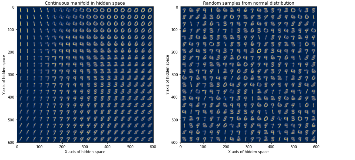
For fig2, I have sampled \(20X20\) random points from \(N\sim(0,1)\) . When we map these points back to the original space, we can see that each of those points seem to represent an image similar to that from the training set. It is important to note here that these are entirely new images generated by the network and are not part of the training set.

For fig1, I have taken $20$ equally spaced points between \(x=[-2,2]\) and similarly \(20\) spaced points between \(y=[-2,2]\). I have used these points to construct a \(20X20\) so that I can visualize the hidden manifold. We can see that the manifold found out by VAE is continuous. The transition between different points in hidden space is very smooth. For example, observe the transition from \(9\;to\;8\), we can see that the manifold is rather continuous.

8.2) Visualization 2: Let’s now visualize how changing the hidden dimension,changes the generated samples.

Like in previous visualization, I have sampled random points from univariate normal distribution.(Instead of sampling points from multivariate gaussian, we can sample from univariate gaussian because we had taken hidden random variables to be independent of each other i.e. covariance matrix was an \(Identity \; Matrix\)).

Variation in generated samples as we change hidden space dimensionality

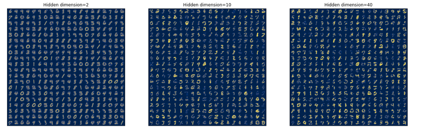
We can observe that, when the hidden dimensionality is 2, the generated samples are quite blurred. As we increase the dimensionality to 10, the generated samples are more sharp. This is due to the fact that when we mapped our data in higher dimension, our network was able to learn some other properties of the data such as sharpness rather than just learning orientation of edges. As we increase the dimensionality further, we can observe that the generated samples contain many points which are hard to decode. This means, that when dimensionality is increased to 40, our decoder network is not able to decode the hidden vectors properly. It maps hidden data points to locations in original space which do not correspond to any digits. If we increase the number of layers in our Neural Network, we can generate extremely good samples even with high dimensional latent space.

8.3) Visualization 3 : Let’s now consider the effect of Reconstruction Loss term and Regularizer term.

For the following results, I have used VAE loss as

\[\begin{equation} Loss = \alpha(Reconstruction\;Loss)+\beta(Regularizer) \end{equation}\]

where I consider different values of \(\alpha\) and \(\beta\) and see how it affects the latent space mapping.(Note: There is this class of VAE’s in which we use \(\beta > 1\). This class of VAE’s are known as \(\beta-VAE\) which I will discuss in some other post.)

Fig. 1 and Fig. 2 in below plots was generated in the same way as explained above. For Fig. 3 , I took \(1000\) data points from the test set and visualized how were they mapped in the latent space.

Considering only Reconstruction Loss term

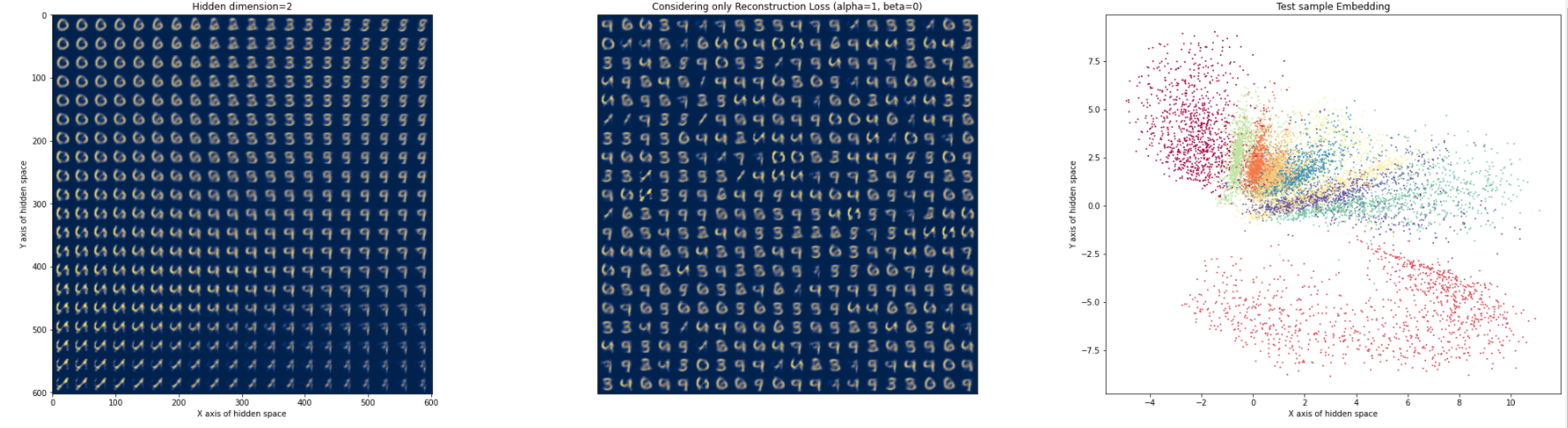
1. Let’s first consider, what happens when only the Reconstruction Loss term is used \((\alpha=1, \beta=0)\) as the VAE Loss function. In this case, we are essentially treating VAE as simple autoencoder which just tries to minimize the errors between generated samples. In this case our VAE Loss becomes almost same as the Autoencoder loss, except the fact that each data point is mapped in such a way that the distribution of points in hidden space will be normal. Also, we can expect that different data points(different digits) will be mapped to different gaussians in the hidden space. Note- In this case, we had no constraint to keep the manifold continuous.

   Considering only KL Divergence Term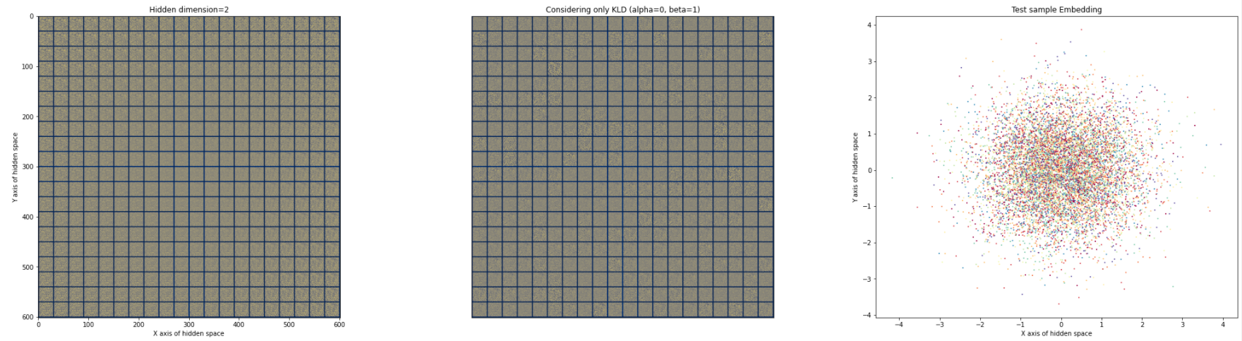
   

2. In second case, we will consider only the Regularizer term\((\alpha=0,\beta=1)\) . In this case, we are not doing anything useful. When we don’t consider the Reconstruction Loss term,we are essentially not training our decoder at all. We are just generating random samples from \(N\sim(0,1)\) and passing mapping it to some arbitrary space using random decoder weights. Therefore we observe noise in fig1 and fig2. Also, since we are just focusing on making posterior \(q(Z/x)\) to be exactly same as \(P(Z)\), we are not retaining any useful information during our mapping. Therefore, we can see all test data points being mapped to \(N(0,1)\) in hidden space without any meaningful structure.

   Considering bothReconstruction Loss and KL Divergence Term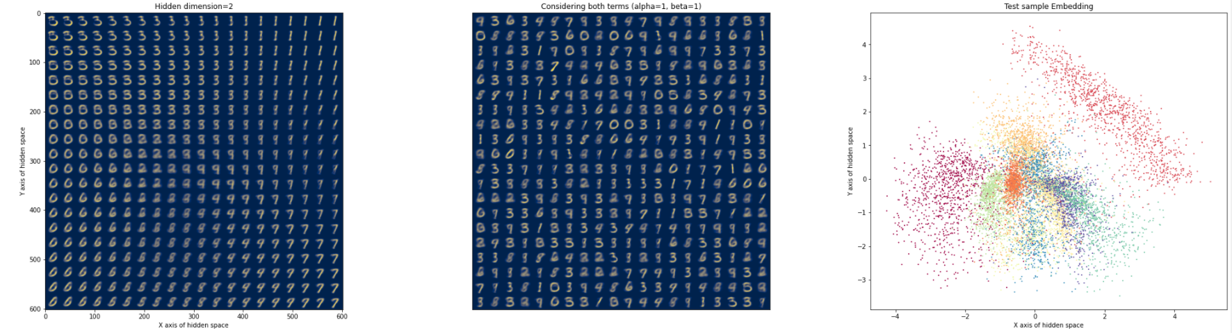
   

3. In third case, we consider both the terms and the results are as we expected. A continuous manifold in hidden space(fig.1) and when test data points are mapped to latent space we can observe continuous transition between different regions(fig. 3)